Rolph Recto - Home Blog

Stack Graphs via CFL Reachability

February 16, 2026

The stack graphs framework is a neat technology from GitHub that allows for name resolution in a language-independent way. The idea is you build a graph from ASTs, and then compute paths over this graph to do name resolution.

Stack graphs build on scope graphs from Eelco Visser’s group at TU Delft, but with some changes to allow for scalable name resolution. As their name implies, stack graphs allow deferred name resolution: a use of a symbol pushes to the stack, and definitions for the symbol pop from the stack. Thus in stack graphs paths from uses to defs can be computed by a graph reachability query, with the added constraint that the nodes along the path maintain stack discipline. This stack structure allows name resolution queries to be incremental, as we will see below.

I was trying to understand the algorithm for how names are resolved and it seemed familiar. Then I realized why: you can view stack graphs as yet another instance of CFL reachability in program analysis. If we can compute name resolution queries in stack graphs by CFL reachability queries, then we can use the wide range of existing tools for CFL reachability to compute these queries for free.

Stack Graphs

First, let’s do a quick recap of stack graphs by going through an example from the stack graphs paper from 2023. Here are two Python files, a.py and b.py.

# a.py
class A:
    x = 0

# b.py
from a import *

class B(A):
    pass
    
print(B.x)
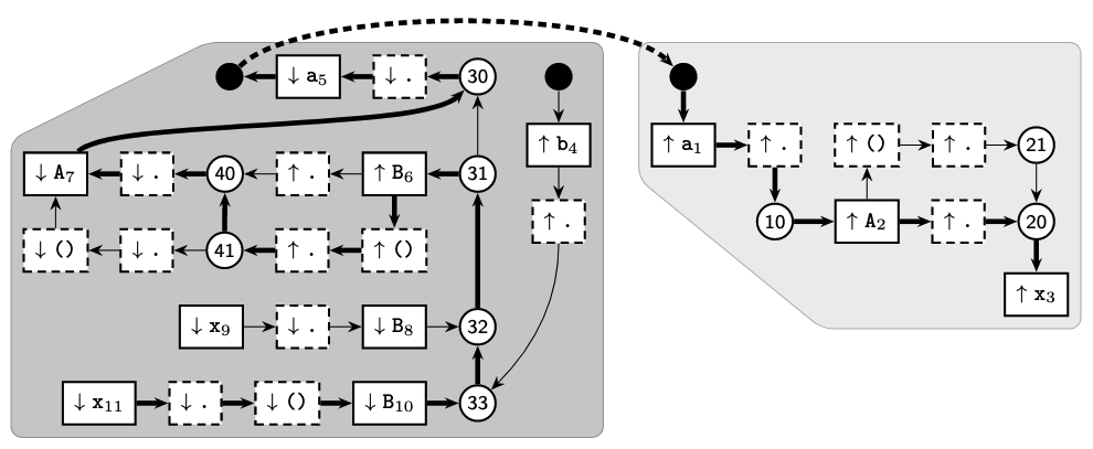
print(B().x)

The stack graph for these two files is shown below.

Stack graph example; from Figure 3 of the Stack Graphs paper

The b.py section of the graph is the darker shaded section on the left, while the a.py section of the graph is the lighter shaded section to the right. Note that every symbol use and def is made unique: thus the x in B().x becomes x11, and so on. The black circles represent “root” nodes, which can represent either the “root” scope for a file or imports. These are the only nodes that can connect the parts of the stack graph that represent different files. Square nodes that represent symbol uses have labels that begin with a down arrow (↓), while nodes that represent symbol definitions have labels that begin with an up arrow (↑). Circle nodes represent lexical scopes.

Let’s focus on the b.py section of the graph. The nodes at the bottom-left starting from x11 through B10 represent the expression B().x, while the nodes x9 through B8 represent the expression B.x. The two rows of nodes above these, which contain B6 and A7, represent the definition of class B. The nodes around a5 represent the import statement at the top of b.py, while the nodes around b4 represent the module b.py; other modules that import from b.py will generate paths that traverse this part of the graph.

The graph above highlights a path from x11 to x3, which represents the resolution of the x symbol in print(B().x) to the class attribute x defined in class A. Here is a detailed description from the Stack Graphs paper:

We start with an “empty” path from x11 to itself. With each step, we append an edge to the path, and show the path’s current frontier and the stack of currently pending lookups. This stack contains both program identifiers (e.g. x) indicating names that we need to resolve, and operators (e.g. .) indicating how the resolved definitions will be used. Whenever we encounter a reference or push node, we prepend the node’s symbol to the stack. Whenever we encounter a definition or pop node, we verify that the stack starts with the node’s symbol, and remove it from the stack. The final name binding path ends at a definition node and has an empty stack, indicating that there are no more pending lookups, and the name binding path is complete.

The design of stack graphs allows for scalable name resolution because they allow for incremental updates whenever a file changes. Instead of recomputing all paths whenever a file changes, which would be prohibitively expensive if a code repository is big, instead only paths within the section of the stack graph corresponding to the changed file. This is easy to do because all cross-file paths must go through root nodes (i.e. black circles in the example above). Because of this feature, the stack graphs implementation can compute partial paths at index time for intra-file sections of the stack graph to speed up path computations at query time.

CFL reachability

CFL reachability is basically graph reachability with a twist: given a context-free language \(L\) and a graph \(G\) such that edges of the graph are labeled with terminals drawn from the alphabet \(\Sigma\) of \(L\), we want to determine whether for a pair of nodes there exists a path through \(G\) such that the word formed by concatenating the terminals along the edges of the path is in \(L\). CFL reachability is quite popular in program analysis, as you can encode many program analyses as CFL reachability queries. See this paper by Tom Reps to get an overview.

The most common context-free languages used in CFL reachability in program analysis are the Dyck languages, or the language of balanced parentheses. Dyck-1, for example, has only one kind of parenthesis in its alphabet; Dyck-\(n\) in general has \(n\) different kinds of parentheses in its alphabet. Dyck-1 accepts strings such as (), (()), ()(), and so on; but not strings such as ((, )(, ((). Consider the graph below, where the edges are labeled with parentheses.

From node A, node E is not CFL-reachable (even though it is reachable in the normal sense) because the two paths from A to E are labeled (() and ()( respectively, neither of which are in Dyck-1. From node B, however, node E is CFL-reachable because the path B -> D -> E is labeled with word (), which is in Dyck-1.

Stack Graphs to CFL Graphs

How do we convert a stack graph to a “CFL graph” amenable to CFL reachability queries? This is surprisingly easy. The CFL graph keeps the same nodes and edges of the stack graph; after that, the only thing left to do is to add labels on the edges, where the labels are characters of the alphabet of some CFL. The following simple rules define edge labels.¹

for push nodes in the stack graph, decorate all the node’s outgoing edges with the node’s label.
for pop nodes in the stack graph, decorate all the node’s incoming edges with the node’s label.
decorate all other edges with a “no-op” (\(\circ\)) label

Conversion from stack graph (green) to CFL graph (blue)

So we have a stack graph converted into a CFL reachability problem. How are we going to compute CFL reachability? It is common in program analysis to use the tabulation algorithm from the IFDS paper to compute CFL reachability, which you can think of as a variant of the CYK parsing algorithm. Today, however, we’re going a different route and instead exploit a neat property of CFL reachability: you can solve it using a Datalog program² that closely mirrors the grammar of the context-free language. This gives a few advantages when we compute stack graphs via CFL reachability.

This approach allows stack graphs to be incrementally updated, provided the Datalog engine we use supports incremental computation, as in Differential Datalog).
The output database / IDB of the Datalog program naturally already contains parsing information that corresponds to partial paths, which allow you to move computation from query time to index time. (See the Stack Graphs paper for more information.)
You can write a query to only resolve a specific use of a variable by transforming the Datalog program into a “demanded” version, which will be faster to evaluate than the exhaustive version that resolves all variable uses.

Note that the original stack graphs approach already had the first two features, but here we get them for free just by using Datalog.

Before we get to the Datalog program though, we need to define the grammar of the context-free language that we’re using, Dyck-\(n\). Let \(S\) be a set of \(n\) symbols. Given \(1 \leq i \leq n\), the Dyck-\(n\) language has the following grammar, where \((_\textup{i}\) only matches with \()_\textup{i}\) . \[ \begin{align} \textup{S} & \leftarrow \epsilon \mid (_\textup{i} \; \textup{S} \; )_\textup{i} \mid \textup{S} \; \textup{S} \end{align} \] Note that open parens correspond to push operations, while close parens correspond to pop operations. Thus you can take the terminal \(\downarrow_{\textup{i}}\) as an operation that pushes the symbol \(S_\textup{i}\) to the stack, while \(\uparrow_{\textup{i}}\) is an operation that pops \(S_\textup{i}\) from the stack. The fact that Dyck languages only accept strings of balanced parentheses means that an accepted string maintains proper stack discipline—exactly the constraint we need to enforce for paths in a stack graph.

The grammar above is close but not quite what we need, because we also have to deal with no-op labels for edges, not just pushes and pops. Here is another pass at the grammar, this time taking account of no-ops (marked \(\circ\) in the grammar). The idea is that parentheses can be surrounded by any symbol of \(\circ\) symbols and it would still be parsed effectively the same.

\[ \begin{align} \textup{S} & \leftarrow \epsilon \mid \textup{L}_i \; \textup{S} \; \textup{R}_i \mid \textup{S} \; \textup{S} \\ \textup{N} & \leftarrow \epsilon \mid \circ \mid \textup{N} \; \textup{N} \\ \textup{L}_i & \leftarrow \textup{N} \; (_\textup{i} \; \textup{N} \; \\ \textup{R}_i & \leftarrow \textup{N} \; )_\textup{i} \; \textup{N} \\ \end{align} \] Now let’s write a Datalog program to capture this grammar. The idea is to have a relation correspond to every terminal and nonterminal in the grammar, and a Datalog rule to correspond to every grammar production rule.

Let’s first represent nodes and edges of the stack graph. Note that I’m using Souffle Datalog syntax.

.decl Node(x:symbol, id:symbol, act:symbol)
.decl Edge(id1:symbol, id2:symbol)

The Node relation contains the symbol that the node pushes to the stack (if any), the ID of the node, and the action that the node performs on the stack (push, pop, no-op). The Edge relation represents edges between nodes in the stack graph, and contains the IDs for the source and target nodes.

As an example, let’s represent the nodes and edges along the path from x11 to B10 in the stack graph.

Node("x","x11","PUSH").
Node("$DOT","$DOT100","PUSH").
Node("$CALL","$CALL200","PUSH").
Node("B","B10","PUSH").

Edge("x11","$DOT100").
Edge("$DOT100","$CALL200").
Edge("$CALL200","B10").

Now let’s define the actual grammar. These relations and rules correspond one-to-one with nonterminals and production rules of the grammar. Each tuple \((n_1, n_2)\) in a relation \(R\) represents the existence of a path from node \(n_1\) to node \(n_2\) labeled \(R\), which can be either a terminal or a nonterminal.

.decl S(id1:symbol, id2:symbol)
S(ID,ID) :- Node(_, ID, _).
S(ID1,ID4) :- L(ID1,X,ID2), S(ID2,ID3), R(ID3,X,ID4).
S(ID1,ID3) :- S(ID1,ID2), S(ID2,ID3).

.decl L(id1:symbol, x:symbol, id2:symbol)
L(ID1,X,ID4) :- N(ID1,ID2), Push(ID2,ID3,X), N(ID3,ID4).

.decl R(id1:symbol, x:symbol, id2:symbol)
R(ID1,X,ID4) :- N(ID1,ID2), Pop(ID2,ID3,X), N(ID3,ID4).

.decl F(id1:symbol, id2:symbol)
N(ID,ID) :- Node(_,ID,_).
N(ID1,ID2) :- Nop(ID1,ID2).
N(ID1,ID3) :- N(ID1,ID2), N(ID2,ID3).

Finally, let’s look at the Push and Pop relations, which define how edges are labeled for the CFL graph. These relations use the rules above that convert from the stack graph to the CFL graph.

.decl Push(id1:symbol,id2:symbol,sym:symbol)
Push(ID1,ID2,X1) :-
    Node(X1,ID1,ACT1), Node(_,ID2,ACT2), Edge(ID1,ID2),
    contains("PUSH",ACT1), !contains("POP",ACT2).

.decl Pop(id1:symbol, id2:symbol, sym:symbol)
Pop(ID1,ID2,X2) :-
    Node(_,ID1,ACT1), Node(X2,ID2,ACT2), Edge(ID1,ID2),
    !contains("PUSH",ACT1), contains("POP",ACT2).

.decl Nop(id1:symbol, id2:symbol)
Nop(ID1,ID2) :-
    Node(_,ID1,_), Node(_,ID2,_), Edge(ID1,ID2),
    !Push(ID1,ID2,_), !Pop(ID1,ID2,_).

Finally, we define a relation Out that filters out pairs inS to only return pairs of symbol use-defs. Note that Out(x, y) means that symbol use at node x resolves to the symbol definition at node y.

.decl Out(id1:symbol, id2:symbol)
Out(ID1,ID2) :-
    S(ID1,ID2), Node(_,ID1,ACT1), Node(_,ID2,ACT2),
    contains("PUSH",ACT1), contains("POP",ACT2).

If we run the Datalog program on the stack graph example above, the Out relation should return the follow name resolution results:

a5 resolves to a1
B8 resolves to B6
B10 resolves to B6
A7 resolves to A2
x9 resolves to x3
x11 resolves to x3

which is what we expected from the original stack graph name resolution query. You can see the full Datalog program in this gist and run it on Souffle to confirm the results.

That’s it! We’ve successfully computed name resolution from a stack graph using a Datalog program containing a CFL reachability query. Once again CFL reachability proves to be useful for a program analysis task.

What happens when a push node has an edge to a pop node in the stack graph? That would imply the edge has multiple labels. However, this is actually made impossible by the rules of the stack graph’s construction. There should always be a no-op node between a push node and a pop node, so this issue never arises.↩︎
More specifically a “chain” Datalog program. Just look at the example and you’ll see why.↩︎